44 how to show labels in excel chart
How to create a chart with both percentage and value in Excel? In the Format Data Labels pane, please check Category Name option, and uncheck Value option from the Label Options, and then, you will get all percentages and values are displayed in the chart, see screenshot: 15. How to show data label in "percentage" instead of - Microsoft Community Select Format Data Labels. Select Number in the left column. Select Percentage in the popup options. In the Format code field set the number of decimal places required and click Add. (Or if the table data in in percentage format then you can select Link to source.) Click OK. Regards, OssieMac. Report abuse.
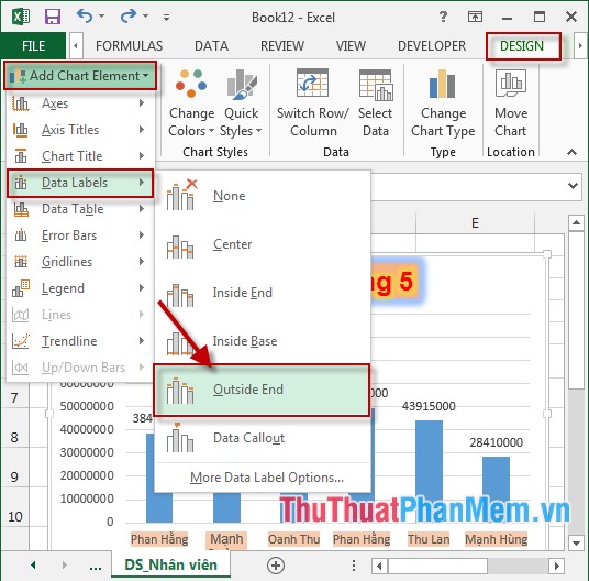
How to Add Data Labels to an Excel 2010 Chart - dummies Click anywhere on the chart that you want to modify. On the Chart Tools Layout tab, click the Data Labels button in the Labels group. A menu of data label placement options appears: None: The default choice; it means you don't want to display data labels. Center to position the data labels in the middle of each data point.

How to show labels in excel chart
How to Insert Axis Labels In An Excel Chart | Excelchat We will go to Chart Design and select Add Chart Element Figure 6 - Insert axis labels in Excel In the drop-down menu, we will click on Axis Titles, and subsequently, select Primary vertical Figure 7 - Edit vertical axis labels in Excel Now, we can enter the name we want for the primary vertical axis label. How to Show Pie Chart Data Labels in Percentage in Excel Firstly, click as follows: Chart Design > Quick Layout. Then select a layout that has data labels in percentage. I chose Layout 1. Then you will see that the layout is showing the percentage in data labels along with the chart title. 3. Using Format Data Labels to Show Data Labels in Percentage Unable to see the Label Position in excel chart. You can set the position of a label first, then click Label Options > Data Label Series > Clone Current Label to quickly apply custom data label formatting to the other data points in the series. Best regards, Jazlyn ----------- •Beware of Scammers posting fake Support Numbers here.
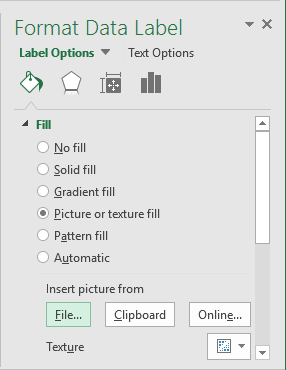
How to show labels in excel chart. Change the format of data labels in a chart To get there, after adding your data labels, select the data label to format, and then click Chart Elements > Data Labels > More Options. To go to the appropriate area, click one of the four icons ( Fill & Line, Effects, Size & Properties ( Layout & Properties in Outlook or Word), or Label Options) shown here. Change the format of data labels in a chart - Microsoft Support You can make your data label just about any shape to personalize your chart. Right-click the data label you want to change, and then click Change Data Label ... Dynamically Label Excel Chart Series Lines - My Online Training Hub Step 1: Duplicate the Series. The first trick here is that we have 2 series for each region; one for the line and one for the label, as you can see in the table below: Select columns B:J and insert a line chart (do not include column A). To modify the axis so the Year and Month labels are nested; right-click the chart > Select Data > Edit the ... How to Add Axis Labels in Excel Charts - Step-by-Step (2022) How to add axis titles 1. Left-click the Excel chart. 2. Click the plus button in the upper right corner of the chart. 3. Click Axis Titles to put a checkmark in the axis title checkbox. This will display axis titles. 4. Click the added axis title text box to write your axis label.
How to rotate axis labels in chart in Excel? - ExtendOffice If you are using Microsoft Excel 2013, you can rotate the axis labels with following steps: 1. Go to the chart and right click its axis labels you will rotate, and select the Format Axis from the context menu. 2. How to add or move data labels in Excel chart? - ExtendOffice In Excel 2013 or 2016. 1. Click the chart to show the Chart Elements button . 2. Then click the Chart Elements, and check Data Labels, then you can click the arrow to choose an option about the data labels in the sub menu. See screenshot: In Excel 2010 or 2007. 1. click on the chart to show the Layout tab in the Chart Tools group. See ... Add or remove data labels in a chart - support.microsoft.com Click Label Options and under Label Contains, select the Values From Cells checkbox. When the Data Label Range dialog box appears, go back to the spreadsheet and select the range for which you want the cell values to display as data labels. When you do that, the selected range will appear in the Data Label Range dialog box. Then click OK. How to Create a Bar Chart With Labels Inside Bars in Excel In the Format Data Labels pane, under Label Options selected, set the Label Position to Inside End. 9. Next, in the chart, select the Series 2 Data Labels and then set the Label Position to Inside Base. 10. Then, under Label Contains, check the Category Name option and uncheck the Value and Show Leader Lines options. 11.
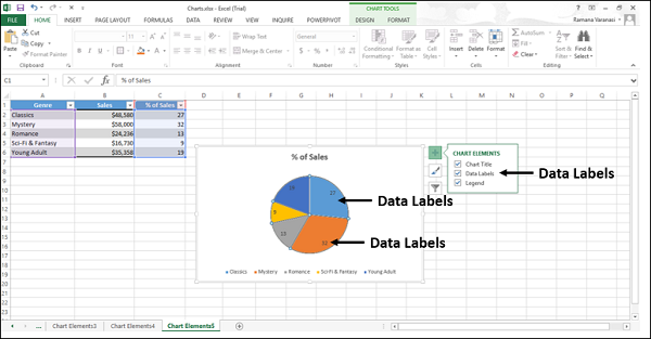
Excel Charts: Dynamic Label positioning of line series - XelPlus Show the Label Instead of the Value for Actual · Select your chart and go to the Format tab, click on the drop-down menu at the upper left-hand portion and ... How to Place Labels Directly Through Your Line Graph in Microsoft Excel Right-click on top of one of those circular data points. You'll see a pop-up window. Click on Add Data Labels. Your unformatted labels will appear to the right of each data point: Click just once on any of those data labels. You'll see little squares around each data point. Then, right-click on any of those data labels. How to add data labels from different column in an Excel chart? Click any data label to select all data labels, and then click the specified data label to select it only in the chart. 3. Go to the formula bar, type =, select the corresponding cell in the different column, and press the Enter key. See screenshot: 4. Repeat the above 2 - 3 steps to add data labels from the different column for other data points. Excel Pie Chart Labels on Slices: Add, Show & Modify Factors When you check the Data Labels option on the Chart Elements icon, it will automatically show the values. However, if the values are not showing, then double-click on the data labels on the pie chart. As a result, a side window called Format Data Labels will appear. Now, go to the drop-down of the Label Options to Label Options tab.
Teach Besides Me: Data Labels Excel 2010
How to Use Cell Values for Excel Chart Labels Select the chart, choose the "Chart Elements" option, click the "Data Labels" arrow, and then "More Options." Uncheck the "Value" box and check the "Value From Cells" box. Select cells C2:C6 to use for the data label range and then click the "OK" button. The values from these cells are now used for the chart data labels.
34 What Is A Data Label In Excel - Labels Niche Ideas
how to add data labels into Excel graphs Feb 10, 2021 — Right-click on a point and choose Add Data Label. You can choose any point to add a label—I'm strategically choosing the endpoint because that's ...
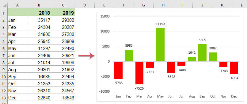
Quickly Create A Year Over Year Comparison Bar Chart In Excel
How to Add Labels to Show Totals in Stacked Column Charts in Excel In the chart, right-click the "Total" series and then, on the shortcut menu, select Add Data Labels. 9. Next, select the labels and then, in the Format Data Labels pane, under Label Options, set the Label Position to Above. 10. While the labels are still selected set their font to Bold. 11.
Creating a simple competition chart - Microsoft Excel 2016
Add a DATA LABEL to ONE POINT on a chart in Excel Steps shown in the video above: Click on the chart line to add the data point to. All the data points will be highlighted. Click again on the single point that you want to add a data label to. Right-click and select ' Add data label ' This is the key step! Right-click again on the data point itself (not the label) and select ' Format data label '.

34 Label Chart In Excel - Labels Database 2020
How to Create a Bar Chart With Labels Above Bars in Excel In the Format Data Labels pane, under Label Options selected, set the Label Position to Inside End. 16. Next, while the labels are still selected, click on Text Options, and then click on the Textbox icon. 17. Uncheck the Wrap text in shape option and set all the Margins to zero. The chart should look like this: 18.

How to Create a Pie Chart in Microsoft Excel
Excel tutorial: How to use data labels Generally, the easiest way to show data labels to use the chart elements menu. When you check the box, you'll see data labels appear in the chart. If you have more than one data series, you can select a series first, then turn on data labels for that series only. You can even select a single bar, and show just one data label.

Create a Line Chart in Excel - Easy Excel Tutorial
How to add axis label to chart in Excel? - ExtendOffice You can insert the horizontal axis label by clicking Primary Horizontal Axis Title under the Axis Title drop down, then click Title Below Axis, and a text box will appear at the bottom of the chart, then you can edit and input your title as following screenshots shown. 4.

Excel chart not printing correctly - i have a simple excel file (office
Edit titles or data labels in a chart - support.microsoft.com On a chart, click the label that you want to link to a corresponding worksheet cell. On the worksheet, click in the formula bar, and then type an equal sign (=). Select the worksheet cell that contains the data or text that you want to display in your chart. You can also type the reference to the worksheet cell in the formula bar.

data visualization - How do you put values over a simple bar chart in Excel? - Cross Validated
Add or remove titles in a chart - Microsoft Support Add a chart title · In the chart, select the "Chart Title" box and type in a title. · Select the + sign to the top-right of the chart. · Select the arrow next to ...

34 What Is A Category Label In Excel - Labels Design Ideas 2020
How to Add Labels to Scatterplot Points in Excel - Statology Step 3: Add Labels to Points. Next, click anywhere on the chart until a green plus (+) sign appears in the top right corner. Then click Data Labels, then click More Options…. In the Format Data Labels window that appears on the right of the screen, uncheck the box next to Y Value and check the box next to Value From Cells.

35 Label In Excel Definition - Labels Database 2020
How To Create Labels In Excel - midtownphillips Link chart title to dynamic text label: Create labels from excel in a word document. All words describing the values (numbers) are called labels. Excel labels, values, and formulas. Click finish & merge in the finish group on the mailings tab. Select mailings > write & insert fields > update labels.

charts - How to change interval between labels in Excel 2013? - Stack Overflow
How do you add data labels to a chart in Excel? | AnswersDrive To format data labels in Excel, choose the set of data labels to format. To do this, click the "Format" tab within the "Chart Tools" contextual tab in the Ribbon. Then select the data labels to format from the "Chart Elements" drop-down in the "Current Selection" button group.

How-to Display Metrics Data in an Excel Dashboard Chart - YouTube
Excel charts: add title, customize chart axis, legend and data labels Click anywhere within your Excel chart, then click the Chart Elements button and check the Axis Titles box. If you want to display the title only for one axis, either horizontal or vertical, click the arrow next to Axis Titles and clear one of the boxes: Click the axis title box on the chart, and type the text.

How to make a pie chart in Excel
Unable to see the Label Position in excel chart. You can set the position of a label first, then click Label Options > Data Label Series > Clone Current Label to quickly apply custom data label formatting to the other data points in the series. Best regards, Jazlyn ----------- •Beware of Scammers posting fake Support Numbers here.
How to Add Labels to an Excel 2007 Chart - Bright Hub
How to Show Pie Chart Data Labels in Percentage in Excel Firstly, click as follows: Chart Design > Quick Layout. Then select a layout that has data labels in percentage. I chose Layout 1. Then you will see that the layout is showing the percentage in data labels along with the chart title. 3. Using Format Data Labels to Show Data Labels in Percentage

Add label to Excel chart line • AuditExcel.co.za
How to Insert Axis Labels In An Excel Chart | Excelchat We will go to Chart Design and select Add Chart Element Figure 6 - Insert axis labels in Excel In the drop-down menu, we will click on Axis Titles, and subsequently, select Primary vertical Figure 7 - Edit vertical axis labels in Excel Now, we can enter the name we want for the primary vertical axis label.
35 Label Definition Excel - Labels For Your Ideas
Post a Comment for "44 how to show labels in excel chart"